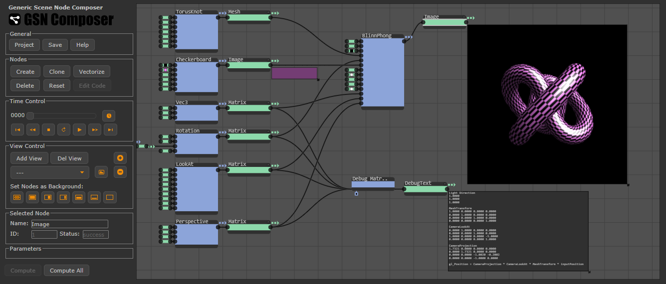
Getting Started | GSN Composer | Online Node-based Visual Programming

Getting Started with the

The GSN Composer is a web-based application that allows rapid interactive creation of programs by connecting nodes using a visual interface.

Why should I get started?

The following features can make the GSN Composer a valuable tool for educators, artists, researchers, or anyone who likes to explore or create interactive demonstrations:

Rapid and intuitive. A user can instantiate ready-made nodes that provide certain functionalities and can connect their inputs and outputs to create a more complex novel functionality. Creating such a composition is very fast and intuitive because it is comparable to sketching a block diagram of a system on a piece of paper when brainstorming, analyzing a problem, or explaining parts of a system and their interactions.
Interactive. The composer is designed for interactivity. It is possible to change certain types of input parameters (called "public parameters") at run-time and observe the effect that the change has on the outputs of the nodes. The input parameters can also be changed automatically over time in a user-defined way, which can create interesting interactive demonstrations.
Programming without coding. The GSN Composer has a visual programming interface that does not require any coding experience. However, users with programming skills can write (and debug) JavaScript code using a special node (called "Plugin" node) and extend the existing functionality according to their needs.
WebGL integration. Image processing and 3D operations that are computationally demanding use WebGL for GPU acceleration. The existing functionality can be extended by custom GLSL shader plugin nodes.
Web Audio and MIDI. The provided audio processing nodes allow working with music and sounds. The GSN Composer can be used as a modular synthesizer that is controllable by external MIDI hardware or its own virtual MIDI devices.
Export to your website. Once a project is created within the composer, the result can be exported as a stand-alone application, which runs independent from the GSN Composer, either offline or as part of your own website.
Free of charge. This website and services were created for educational purposes and without any commercial interest. The usage is free of charge for anyone (commercial or non-commercial users).

Creating Nodes

After launching the GSN Composer its user interface appears, as shown below:

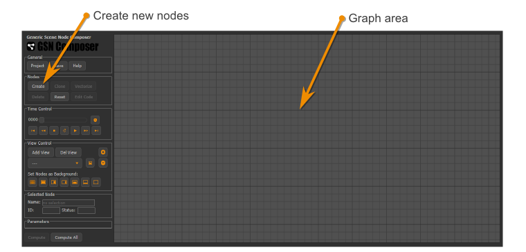
The area with the gray grid on the right is the graph area where the node graph will be displayed. The interface on the left has several operating panels. The panel named Nodes contains a Create button. If you press this button, a dialog appears where you can select the node that you want to create. For each node type, a short description is available. For some nodes, additional information can be found in the documentation.

Once you have selected a node type, the create dialog closes automatically and a new node instance appears in the graph area.

Alternatively, to create a node at a certain position, you can long-press (> 1.5 seconds) with the left mouse button in an empty region of the graph area to open the create dialog.

Moving Nodes and View Navigation

A node in the graph area is selected with a mouse left-click. By pressing the left button and dragging while holding the button down you can move the selected node around.

Possible mouse actions are:

Node selection/motion

Select node: Left-click on node
Move selected node(s): Left-click on a node and dragging while holding
Deselect nodes(s): Left-click and release on the background without motion
Select multiple nodes: Shift + left-click on the node
Area selection: Ctrl + left-click on the background and dragging while holding

View Navigation

Pan the view: Left mouse button press on background or middle mouse button and dragging while holding
Zoom the view: Mouse wheel

The view control panel allows storing the current view using the Add View button. Added views can be restored by selecting them from the drop-down list. It is also possible to render the output of certain nodes in the background of the graph area. To this end, select the nodes that should be displayed and press one of the buttons below the label Set Nodes as Background.

Connecting Nodes to a Graph

There are two basic kinds of nodes: compute nodes and data nodes.

Data nodes store data. They have a green color.
Compute nodes process data. To this end, compute nodes read information from the data nodes at their inputs and write their computed result to the data nodes at their outputs. Compute nodes have a blue color.

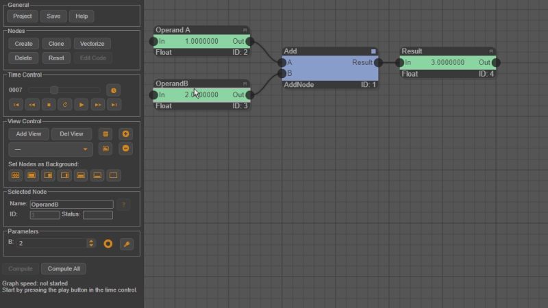
As a simple example, here is a very small graph that adds two numbers:

open example

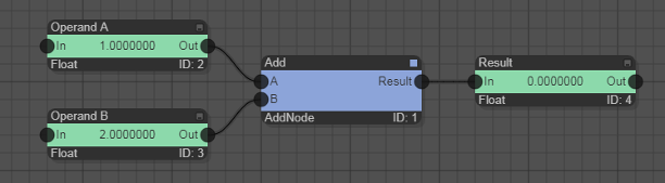
The two input data nodes are the ones on the left side with the values 1.0 and 2.0. The compute node is the blue node in the middle that performs the addition. The output data node is the one on the right, which gets assigned the value 3.0 = 1.0 + 2.0.

Compute and data nodes have to alternate in the graph. This means, a compute node can not be connected to another compute node. Instead, a data node must be placed in between.

Nodes are connected via slots, which are the gray circles at the left and the right side of the nodes. Information is always propagated from left to right through a node, which means slots on the left side of a node are always input slots and slots on the right side are output slots.

Slots are connected by left-clicking on a slot (gray circle). The slot will be highlighted with a yellow color. Now all slots of other nodes that are connectable are also highlighted with a yellow color. By clicking on one of these highlighted slots a connection is established, which is indicated by a black connection line.

Another way to find out which nodes can be connected is to hoover with the mouse over a slot. The node type with which the slot can connect is shown in brackets (e.g. [Float] for a node of type "Float") and in most cases also a short description is given.

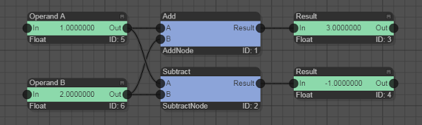
The input and output slots of compute nodes can only have one connection to a data node because a compute node needs to know during computation where to read and write its input and output data. The same is true for the input slot of a data node because with a single connection to a compute node it is ensured that no write-conflict occurs. However, the output slot of a data node can be connected to multiple input slots of one or multiple compute nodes because reading of data can occur in parallel. This is illustrated in the following example, which adds and subtracts the same two data nodes in one time step:

open example

Running the Graph

To start the graph evaluation, the time in the time control panel must be changed, e.g. by pressing the play button or any other available time control element. The graph evaluation takes place in a lazy fashion. This means that the inputs of a compute node are monitored for change and only if a change has occurred, it is executed. Once a compute node has executed, it might change a data node at the output, which can, in turn, trigger the next compute node in the graph to execute during the same time step.

You can overrule the lazy evaluation and force a compute node to execute by selecting a node and pressing the Compute button (or pressing the Compute All button to enforce executing all compute nodes). There are several flags for compute and data nodes that visualize their status:

	Needs compute	A blue square in the upper right corner of a compute node indicates that the lazy evaluation of the node is overwritten and it will execute in the next time step.
	Successful compute	A blue dotted arrow at the upper right corner of a compute node indicates that the compute node has executed and that no error has occurred.
	Failed compute	A red dotted arrow at the upper right corner of a compute node indicates that the compute node has executed and that an error has occurred. Typically, an error message is displayed next to the red arrow.
	Updated data	A green dotted arrow at the upper right corner of a data node indicates that the data node was updated during the last time step.

The "Needs compute" flag of a compute node is sometimes set automatically by the interface. This happens when a compute node was just created (and therefore has never been executed before), when one of its connections has changed, or when a data node at the input was manually changed.

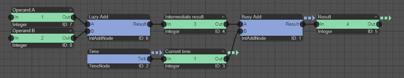
There are some compute nodes that compute in any case. These are for instance nodes that return the mouse position or the current time. Below is an example in which the current time is used as an operand in an addition. Note, how the first addition in the graph is executed only once (lazy evaluation) whereas the second addition is executed in each time step:

open example

Public Parameters

Public parameters are special data nodes. Currently, there are 6 different public parameter types:
[Float], [Integer], [Boolean], [Text], [FileName], and [Color].

Public parameters are special in several ways:

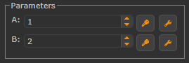
Firstly, public parameters can be changed at run-time. It is often interesting to play around with the parameters and observe the effect the change has on the output of the graph. You can change a public parameter by selecting its node in the graph area. Once selected, an interface element for editing the selected public parameter appears in the Parameter panel. However, the better option is to select a compute node, which has public parameters as inputs. In this case, the interface elements for all input nodes that are public parameters are shown in the Parameter panel. If you hover the mouse over a parameter's interface element, a tooltip is shown with a description of the functionality of the public parameters for the selected compute node.

Secondly, the content of public parameters is stored together with the graph when the graph is saved. Thus, the parameters' content is perfectly restored when the graph is loaded. In contrast, other data nodes, such as images or audio signals, are not stored together with the graph and are not automatically restored when the graph is loaded. However, if the graph structure that generated these volatile data nodes in the first place does still exist, their content will be typically re-created once the graph is run (see also Managing the Project and its Resources).

Thirdly, public parameters can be changed automatically over time in a user-defined way, which can create interesting interactive demonstrations. To this end, the user has the option to set keyframes by pressing on the small button with the key symbol next to the public parameters (see below).

If the keyframe symbol is pressed at a certain time step (which can be selected with the time control panel) the current value of the public parameter is associated with that keyframe time and the node's value is restored automatically if the particular keyframe time is reached again. By setting multiple keyframes at different points in time interesting keyframe animations can be created. The small button with the wrench symbol next to the keyframe button opens a dialog that allows editing the keyframe animation by changing the interpolation type or by deleting unwanted keyframes. The keyframe information is stored together with the graph and is therefore always automatically restored if the graph is loaded. Time steps (also called ticks) are freely configurable. Their duration as well as start and end can be edited by pressing the small button with the clock symbol in the time control panel.

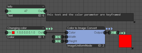
Here, is a simple example for an automated change of public parameters (of type [Text] and [Color]) using keyframes:

open example

Node Hierarchy

Nodes can be arranged in a tree hierarchy. Compute nodes of type Container can have other compute and data nodes as children. Data nodes can have data nodes as children. To make a node a child, drag it while the left mouse button is pressed over the new parent node. If two black downward pointing arrows are displayed, release the mouse button. To detach a node from a parent, move it either upwards or to the left until two black upward-pointing arrows are displayed and release the mouse button. The animation below shows an example where a data node is made a child of a compute node and afterwards is detached again:

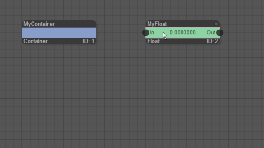
The above example uses a compute node of type Container. A container is special because it has no functionality on its own. Its sole purpose is to structure other nodes hierarchically. This is very useful for grouping nodes and the reduction of a graph's visual complexity.

Another option to simplify the visualization of a graph is to attach data nodes to compute nodes. This is achieved by pressing the small gray minimize icon in the upper right corner of a data node. Technically, this makes the data node a child of the compute nodes. However, the visualization of attached nodes is different to normal child nodes because an attached node will be displayed as a very small green capsule that always sticks right next to its corresponding slot and moves along with its compute node.

For convenience, when creating a new compute node, the GSN Composer automatically creates attached data nodes for required public parameters at the input slots. Furthermore, for all output slots, a corresponding data node is created. However, these data nodes are not always attached automatically but can be attached by the user if desired.

If, at some point, a slot of a compute node is not connected to a data node, an attached data node can be simply created by a long press (> 1.5 seconds) with the left mouse button on an input or output slot of a compute node.

Managing the Project and its Resources

For a very simple graph that does not require additional resources (such as images or audio files) it is not necessary to setup a project unless you want to save or export your graph.

To create (or open) a project press the Project button in the General panel. Here you can enter a project name and create a new project or open an existing one.

In the Save current graph section of the project dialog, a name for the current graph can be set and when the Save button is pressed the graph is saved to the currently opened project. A project can contain multiple graphs. Existing graphs with the same name will be overwritten without a warning.

The Project resource section enlists all available resources of the project, such as graphs, images, or audio files. You can upload your own files from your computer as project resources by pressing the Upload Resources button. It is also possible to drag & drop files directly into the graph area. Supported files types are: image/jpeg, image/png, image/hdr, image/pfm, audio/wav, video/mp4, and model/3d-wavefront-obj. Existing resources with the same name will be overwritten without a warning.

To open an existing graph select the Open action in the project resource list. Another option is to Insert a graph, which does not delete the current graph in the graph area but merges the selected graph into the existing one.

If you want to copy a graph into another project, open the graph, close the current project by pressing Close Project, open the target project, and save the graph with a chosen name. If you want to copy other resources, you need to download them from the source project by pressing the Download action in the resource list and upload them to the target project.

If you want to copy a complete project, first open the project that you want to copy. Then press the Clone Project button in the project dialog and enter a new project name. This way you can make personal copies of existing examples that you can freely modify.

Exporting the Project as a Website

A graph can be exported as a stand-alone application, which runs independent from the GSN Composer, either offline or as part of another website. To this end, a graph must be saved in a project as described in the section above. Then by pressing the Export as Website button in the project dialog a zip package is created and offered as a download. Unzip the package and in the created directory all required files can be found. If the file index.html is opened in a web browser, there should be one graph area shown for each graph in the project. All graphs start their playback automatically. Please refer to the comments in index.html to learn how to resize the graph area, how to start and stop the graph, and how to change a public parameter from your website.

If you open index.html locally on your computer and the graph requires additional resources, such as images or audio files, you might get an error message because cross-origin requests are not supported for the local file:// protocol scheme for most browsers (at least not by default). In this case, you need to place all files from the directory on a (local) web server and access them with the http:// or https:// protocol scheme.

Publishing the Project

Another option to make a project visible to the outside world is to set it to "public". This is achieved by pressing the Make Public button in the project dialog.

If you make your project public, any included graph can be directly opened from anywhere with the URL address:

https://www.gsn-lib.org/index.html#projectName=[yourProjectName]&graphName=[yourGraphName]

Simply share your unique link if you want to use your graph in online presentations, forum discussions, email correspondence, etc.

Optionally, you can request for your project to be included in the GSN Composer gallery. You can check how your graph will look in the gallery by following the link "PreviewExport" that is displayed after each graph in the project resources.

Projects that are public can not be modified anymore. This means, a graph can still be opened and edited but can not be saved under the same project name. Also, other resources in the project, such as images or sound files, can no longer be modified. However, resources can still be downloaded or the complete project can be cloned by pressing the Clone Project button in the project dialog. By cloning a public project it becomes editable again under a different project name.

As all graphs within a public project are reachable by anyone, it is important that you make sure that their content is not harmful, illegal, offensive, or contains infringements of copyrights. If such content is found, the project will be deleted immediately.

Please mention in the description of the graphs the source and license of included resources that you have not created yourself (e.g., Creative Commons CC0, CC BY, CC BY-NC, etc.). Also mention the Creative Commons license under that you want to publish your graph and own resources (if no information is given, CC0 is assumed). If you choose a license that requires attribution, please do not forget to state your name (or pseudonym).

Making a project public can not be undone as a user. Please contact me if you need support.

Vectorizing Data Nodes

Vectorization of data nodes is a very useful feature of the GSN Composer because it can often simplify the graph's complexity and improve its visualization.

All non-vector data nodes can be vectorized by pressing the Vectorize button in the Nodes panel. The resulting vector is a special data node that has an array of ordered data nodes of the original type as its children. E.g., if a [Float] node is vectorized, a [FloatVector] is created that has ordered [Float] elements as children.

A vector data node can be connected to slots that are usually intended to be connected to their corresponding non-vector data node. E.g., a [FloatVector] can be connected to a compute node slot that expects a [Float].

If at least one non-vector type input slot of a compute node has a vector as an input, the compute node is executed several times within a single time step. More specifically, the compute node is executed N times, where N is the length of the largest vectorized input. If a non-vector type output slot of this compute node has a vectorized output, N children will be created at the output where the N-th child of the output vector stores the result of the computation with the N-th child of the input vector.

This sounds complicated but is easy to work with in practice. Let us consider the simple example from the beginning where we computed 1.0 + 2.0 = 3.0. Starting from this example, the animation below shows how the second operand with value 2.0 can be vectorized by pressing the Vectorize button. A [FloatVector] is created that has the original [Float] data node with value 2.0 as a child. By selecting the [Float] data node and then pressing the Clone button, a copy of the [Float] data node is created that is appended as a child to the [FloatVector]. In the example below, three child nodes are created and are assigned the values 2.0, -3.0, and 7.0. Afterwards, the output data node that holds the result of the addition is also vectorized and the graph is played. After the evaluation, the [FloatVector] at the output has three elements that store the results of the three operations:
3.0 = 1.0 + 2.0
-2.0 = 1.0 + (-3.0)
8.0 = 1.0 + 7.0

Thus, in this example, vectorization allows computing three additions (which would normally require three compute node instances) with only a single compute node instance. If the [FloatVector] is folded by pressing on the small collapse icon below the node, its children are not displayed. By folding the vector nodes, the graph structure of this example becomes as compact as the one of the simple addition example from the beginning.

open example

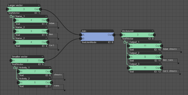
Now, we still need to discuss the case when several non-vector type input slots of a compute node have a vector as an input and these are not of the same size. As stated before, the compute node is always executed N times, where N is the length of the largest vectorized input. Thus, there is missing data if the input vectors have different sizes. As a simple solution, the convention is used that the elements of the smaller vectors are simply re-used starting again from the beginning. As an example, we join a [TextVector] with the elements "Adam", "Ben", and "Carl" with another [TextVector] with the elements " shouts" and " runs". The result is a [TextVector] with three elements "Adam shouts", "Ben runs", and "Carl shouts".

open example

Because vectors hold data nodes and each data node has a considerable memory overhead and computational effort for internal handling, it is not recommended to generate vectors with more than a few dozens of children. E.g., for best performance, instead of creating a very large [FloatVector], a non-vector node of type [Signal] or [Matrix] might be the better choice because these have much less overhead per stored floating-point value.

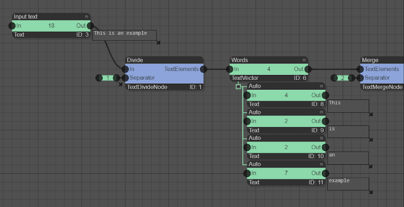
Vector data nodes are not only used for data-parallel feeding of compute nodes. Several compute nodes require a vector data node as regular input or output. Such usage is demonstrated in the example below in which a [Text] node is split into words using space as a separator. The output is a vector of words of type [TextVector]. This vector is then merged again into a single text in which the words are separated by commas.

open example

Creating own Plugin Nodes

If you are familiar with JavaScript, you can create your own compute node and extend the existing functionality of the GSN Composer according to your needs. To this end, an instance of the General.Compute.Plugin node can be created. If you select the plugin node in the graph area, the Edit Code button in the Nodes panel can be clicked. A dialog appears in which you can enter JavaScript code for two functions: init() and run().

The init() function is called when the node is created (or re-created after a code change). Typically, the main purpose of this function is to define which input and output slots are required for your plugin node.
The run() function is called each time an input changes. Typically here the required information is read from the inputs, the result is computed, and the outputs are updated with the new result.

A more detailed discussion, sample code, and instructions on how you can debug your code can be found in the documentation of the General.Compute.Plugin node. There are also several examples that demonstrate its usage.

Furthermore, custom GLSL shader nodes can be added using the ImageProcessing.Compute.Plugin.ImageShader node or the 3D.Compute.Plugin.Shader node.

Currently, the GSN Composer's functional range is still constantly expanding and a suitable node for your particular needs might not yet be included. Therefore, if you are not able to create a Plugin node yourself, you are very welcome to contact me with your request and I will try to create a solution for you.

Loops in the Graph

To evaluate the graph, the order in which compute nodes are executed must be determined. This is only possible if the graph does not contain loops because they would cause a cyclic dependency of nodes. Therefore, if a user tries to add a connection between nodes and this connection would generate a loop, this connection is refused and an error message is shown in the graph area.

Still, it is sometimes desirable to use the result of a previous computation in the next time step. To this end, a General.Compute.DelayedCopy node can be used. This node is special because all nodes of type [DelayedCopy] in a graph will be executed prior to all the other nodes of other types. When executed, a DelayedCopy node makes a copy of any data node that is connected to its input. Thus, though there is a feedback loop between time steps, there is no cyclic dependency for the evaluation in the current time step because it is clear that the evaluation should start from the DelayedCopy nodes and should stop once a DelayedCopy node is reached again. To mark this special behavior visually, connections into DelayedCopy nodes are drawn with dashed lines (open example)

Please use DelayedCopy nodes only if no other options are available. The behavior of a graph becomes less replicable with DelayedCopy nodes because all previous time steps may influence the current results. Because only public parameters are restored when a graph is loaded, it is especially problematic if other data nodes are copied with DelayedCopy nodes because these data nodes might not have valid content when the first copy operation is executed.

Another node that creates (at least visually) a loop in the graph is the Input.Compute.Mouse node. However, the connection to a reference node is only to inform the mouse node whether the mouse position should be given relative to the area where the reference node displays its data. E.g., if an [Image] node is connected, the mouse actions and positions are only captured inside of the displayed image. However, this connection does not create a real cyclic dependency for the evaluation, which is the reason why the connection between a mouse node and a reference node is drawn with a dashed line (open example).

Wireless Connections

For large projects, the node graph's visual complexity can become a significant problem. Especially long node connections between different areas of the graph can be visually distracting. For those connection lines, it might be a good idea to change the connection to a "wireless" connection. This means that the connection is still there, the connection line is simply not fully drawn. Instead, only short wire connections with wireless icons at both ends are shown, where the wireless icons consist of three concentric black circles. To create a wireless connection, you first need to create a regular "wired" slot connection. Then perform a long press (> 1.5 seconds) with the left mouse button on an input or output slot (which are the gray circles at the side of the nodes) to toggle between a wireless and a wired connection.

Wireless connections should be used carefully. They help to reduce the visual complexity but the connection information of nodes is no longer directly visible.