Examples
| Simple | |||
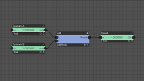 |
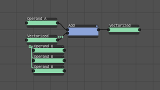
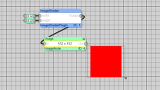
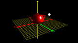
Add | This very simple example adds two floating point numbers | |
 |
AddSub | This example adds and subtracts the same two floating point values in one time step | |
 |
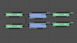
Lazy | In this example, the current time is used as an operand in an addition. Note, how the first addition in the graph is executed only once (lazy evaluation) whereas the second add is executed in each time step. | |
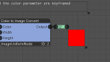 |
Keyframes | This is an example for an automated change of public parameters (of type text and color) using keyframes. | |
| Vectors and Containers | |||
 |
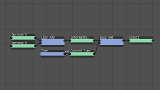
VectorAdd | Vectorization can simplify a graph because many operations of the same type can be executed with a single compute node instance. In this example, an addition is computed for each child of the FloatVector. | |
 |
DifferentSizes | This example demonstrates what happens when a compute node has several vectorized data nodes as an input and these are not of the same size. | |
 |
DivideMerge | This examples divides a text into words using space as a separator. The output of the divide compute node is a vector of words of type [TextVector]. This vector is then merged again into a single text in which the words are separated by commas. | |
 |
Container | Container nodes allow for the hierarchical organization of a graph. As a simple example, the text of a fairytale is structured as a parent container with two child paragraphs, each of which contains two sentences. | |
| Image Compositing | |||
 |
Rocket | In this example, a moving rocket is placed on top of a static background. | |
 |
FollowShape | In this example, several images are moving alone a predefined path (e.g. a circle). | |
 |
Torchlight | This example uses a compositing mask to generate a simple torchlight effect. | |
 |
Accumulate | This example demonstrates the usage of the accumulate node. | |
 |
Tile Map | In this example, it is shown how tiles from a tile map can be composited into a scrollable background image for 2D games. More information about 2D game creation with the GSN Composer is available here. |
|
| Sprite Sheet | This example demonstrates how to composite an image from many sprites defined in a sprite sheet. | ||
| Sprite Grid | This example demonstrates how to generate a scoreboard for a 2D game using the SpriteGrid node. | ||
| 3D | |||
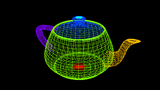 |
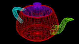
LoadMesh | This example shows how to load a 3D mesh. To learn about 3D rendering with the GSN Composer, you can follow this tutorial. |
|
 |
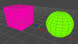
GetGroup | In this example a mesh group is extracted from a mesh. | |
 |
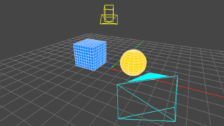
SceneInspector | This example demonstrates the SceneInspector node. | |
 |
DirectionalLight | A directional light and a camera is added to the scene. | |
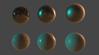 |
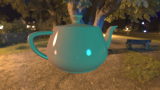
ImageBasedLighting | This example demonstrates how to perform image-based lighting (IBL) using the built-in scene rendering pipeline. | |
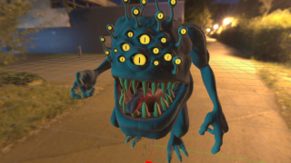 |
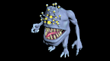
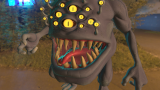
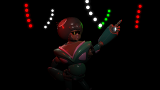
StoneDemonTexture | In this example, several 2D textures are added to a 3D mesh of a stone demon. The scene is rendered using the built-in rasterizer node. | |
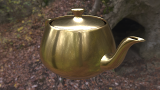
| Transparency | This example showcases different options for the transparency of a 3D surface. | ||
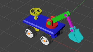 |
Toy Digger | This example shows how to create a scene hierarchy using the merge and similarity nodes. | |
 |
Load glTF | This example demonstrates how to load glTF files using the LoadScene node. Currently, only the GLB binary format is supported. | |
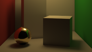 |
Cornell Box | In this example, the built-in raytracer node is is used to render the Cornell box test scene. | |
| Audio | |||
 |
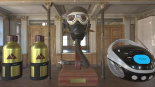
Play Audio File | This example shows how to load an audio file as a signal and start its playback. To learn about audio-related nodes, follow this tutorial. |
|
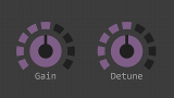 |
AudioBuffer | In this example, an AudioBuffer node is used for stream-based audio playback of a loaded signal. During playback, the gain and detune parameter of the AudioBuffer node can be changed interactively via the provided knobs. | |
 |
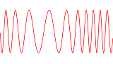
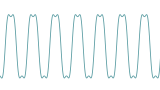
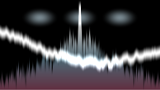
OneOscillator | Probably the most simple setup. A single oscillator is connected via an analyser to the play destination node. | |
 |
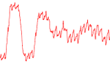
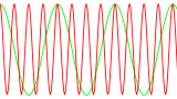
TwoOscillators | This example contains two oscillators that are detuned by 4 cents. Because they have slightly different frequencies, their superposition produces an alternating interference pattern when over time the two waves either double their amplitude or cancel each other out. | |
 |
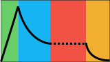
LFO | In this example, the output stream of a low-frequency oscillator (LFO) is connected to the detune input slot of a regular oscillator. | |
 |
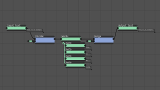
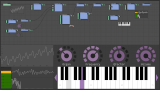
Instrument | This example demonstrates a simplistic instrument build from three oscillators. It can be triggered with a virtual or real midi controller. The "pop" artifacts occur because no amplitude envelope is used. | |
 |
OneEnvelope | A conjoined ADSR envelope is added to the example above, which removes the "pop" artifacts. | |
 |
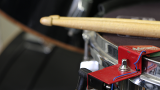
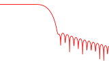
Kick Drum | In this example, a kick drum sound is synthesized by pitch and amplitude modulation of a triangle wave. | |
 |
Piano | An InstrumentMulti node is used as a sample player to create 7 octaves of a piano from a total of 14 audio samples. | |
 |
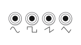
VelSensitivity | Dependent on the velocity of the triggered MIDI key, different sounds are synthesized (sine, triangle, and square wave). | |
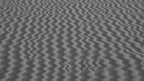 |
FilteredNoise | White noise with a flat spectral density is filtered by a BiquadFilter node. | |
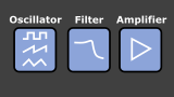 |
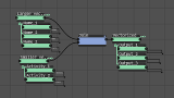
SubtractiveSynth | This example demonstrate how to build a subtractive synthesizer from two oscillators, one noise generator, an LFO, two chained biquad filters, and three ADSR envelopes. | |
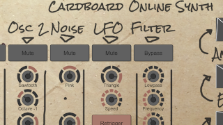 |
CardboardSynth | This example demonstrates how to add a user interface to the subtractive synthesizer from the previous example. It is the visual source code for the Cardboard Online Synth. | |
 |
FM Bells | Bell sounds are a typical example for FM synthesis. A sine modulator changes the phase offset of a sine carrier signal. | |
 |
Wavetable Strings | In this example for wavetable synthesis, two different periodic waveforms are used that are extracted from the recording of a string ensemble. The linear interpolation of the two waveforms is modulated with an LFO. | |
 |
Wavetable Filter | This example demonstrates how to combine a wavetable oscillator with a filter. | |
 |
Periodic Wave | This example shows how to perform additive synthesis with the PeriodicWave oscillator. The individual harmonic components can be interactively edited with the HarmonicWave node. | |
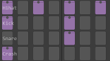 |
Drum Machine Basic | In this example, the step sequencer node is used to generate a simple drum machine from four audio samples. | |
 |
Drum Machine | Drum machine example with funky drum sounds. Sounds can be changed by cloning the project in the project dialog and uploading own audio samples. | |
 |
Rock Drums | Drum machine example with rock drum sounds. | |
 |
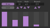
ShortNotes | Musical notes in the step sequencer that are too short to be displayed as regular rounded markers are indicated by triangles with fixed length. | |
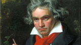 |
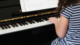
SequencerPiano | A step sequencer node plays the beginning of Beethoven's "Für Elise". | |
 |
Record | The record view of the step sequencer provides the possibility to record the input of a MIDI device, e.g., from a MIDI keyboard controller. | |
 |
SongLoop | In this example, a simple music loop is created from 4 instruments and a step sequencer. | |
| Image Processing | |||
 |
PseudoColor | This example demonstrates how to convert a grayscale image to a color image using a selectable colormap. | |
 |
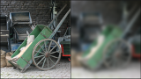
EdgeDetection | In this example, a Sobel filter is used to perform edge detection. | |
 |
Filter3x3 | This example shows how to work with your own custom filter kernels for image filtering. | |
 |
Separable | This example shows how to perform image filtering using custom separable filter kernels. | |
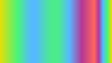 |
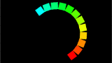
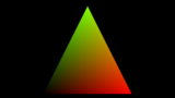
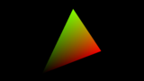
Multi-Gradient | This example demonstrates how to generate a multi-color gradient image. The individual color transitions are controlled via the editable interpolation function. | |
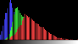 |
Histogram Bars | In this example, a histogram of a selected image region is computed and visualized as a bar chart. | |
 |
Fourier2D | This example demonstrates the usage of a 2D Fourier transform and its inverse to perform image filtering. | |
 |
BatchProcessing | This example shows how to execute several image processing operations on a batch of images. | |
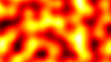 |
PerlinNoise | This example shows how to generate 3D Perlin noise. | |
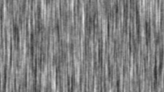 |
Tileable Noise | This example generates tileable noise using the 2D Inverse Discrete Fourier Transform (IDFT). Since the DFT assumes periodic signals, the resulting spatial noise is perfectly seamless. | |
| Signal Processing | |||
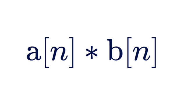 |
Convolution | This example shows how two signals are convolved. | |
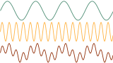 |
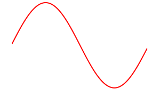
Lowpass | In this example, two sine waves with a lower and a higher frequency are superimposed by an addition. By using a low-pass and a high-pass filter, it is possible to separate the signals again. | |
 |
DFT | In this example, a cosine wave is transformed into the frequency domain by using the discrete Fourier transform (DFT). Afterwards the original signal is recovered with the inverse discrete Fourier transform (IDFT). | |
 |
Frequency Response | This example computes the frequency response of a low-pass filter in decibels. The cut-off frequency of the low-pass filter is changed over time. | |
 |
Custom Filter | This example shows how to apply a custom filter to a signal. | |
 |
Black Box | This example demonstrates a basic finding from signal processing: the response of an LTI system to any input can be determined by convolving the input with the system's impulse response. | |
| Video | |||
 |
MultiMirror | This example shows how to apply a multi-mirror effect on a video. Video source: Big Buck Bunny, Blender Foundation, CC-BY | |
| Paths | |||
 |
MultiplePaths | This example shows how to render multiple paths with different styles into an image (and how to export them as an SVG drawing). | |
 |
PathInterpolation | In this example, an interpolation between two paths is demonstrated. | |
| Apparent Loops | |||
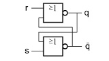 |
FlipFlop | This examples shows how to use the DelayedCopy node to create a simulation of a RS flip flop. General information about flip flops can be found on Wikipedia. | |
 |
FollowMouse | In this example, two images are composited and the foreground image follows the mouse pointer position. | |
| Plugin Node | |||
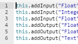 |
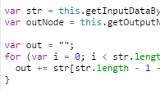
Numbers | This example shows how to work with the plugin node to manipulate float and integer nodes. | |
 |
ReverseText | This examples shows how to reverse a text using the plugin node | |
 |
RandomColorOffset | This examples shows how to work with color nodes using the plugin node | |
 |
Sine | This examples shows how to work with a signal node using the plugin node. | |
| GLSL ImageShader Plugin | |||
 |
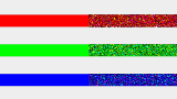
AllRed | A very simple example for a GLSL image shader plugin that sets all pixels to red. To learn about the GLSL ImageShader plugin node, you can follow this tutorial. |
|
 |
TextureCoordinates | In this GLSL example, texture coordinates are introduced. | |
 |
OneBlack | This GLSL example shows how to convert texture coordinates to pixel coordinates. | |
 |
TextureParameter | This GLSL example shows how to change the texture parameters of input images. | |
 |
MouseAsUniform | This example shows how to access the current mouse position from GLSL shader code. | |
 |
JuliaFractal | In this example, the Julia set fractal is computed using GLSL code. | |
 |
AnalyseSound | This example shows how to setup a GLSL ImageShader that reacts to sound input. | |
 |
MultipleOutputs | This example demonstrates how to write a GLSL shader with multiple outputs. | |
 |
ShaderToyInputs | This example shows how to convert the GSN Composer's mouse and time inputs to the input uniform variables expected by a shader from the ShaderToy website. | |
| GLSL Shader Plugin | |||
 |
FirstShader | This example uses a minimalistic shader that renders a mesh with the texture coordinates as colors.
To learn about the GLSL Shader plugin node, you can follow this tutorial. |
|
 |
ShaderUniform | This sample shader introduces a projection and a modelview transformation matrix that are passed as uniform variables. | |
| NormalTrans | In this example, it is shown how mesh normals can transformed with the transposed inverse modelview matrix. | ||
 |
ShaderTexture | This example shows how to access a 2D texture in the shader. | |
 |
ShaderBlinnPhong | This shader example computes Blinn-Phong shading with a directional light. | |
 |
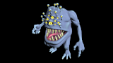
StoneDemonPhong | In this example for a custom 3D shader, a stone demon is rendered with the modified Phong BRDF. | |
 |
StoneDemonPBR | In this example, a stone demon is rendered with the GGX microfacet BRDF. | |
 |
ShaderPhongPointLight | This shader example computes Blinn-Phong shading with a point light. | |
 |
EnvmapLighting | This example shows how to perform image-based environment lighting using the modified Phong BRDF. | |
 |
ImageBasedLighting | This example contains a plugin shader node that performs image-based lighting using the GGX microfacet BRDF. | |
 |
StoneDemonIBL | In this example for a custom 3D shader, a stone demon is rendered with the GGX microfacet BRDF and image-based lighting (IBL). | |
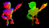 |
DiscoBotDeferred | This example shows how to create a custom GLSL 3D shader that renders positions, normals, and texture coordinates to multiple render targets (MRT) as a prerequisite for deferred shading. | |
 |
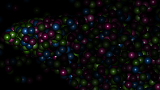
Many Lights | This shader employs multiple render targets for creating a G-Buffer, which is used afterwards for deferred shading with many dynamic point lights. | |
 |
ParticleShader | This is a basic setup for modifying particles with GLSL shaders. Dependent on the capabilities of the employed GPU, several hundred-thousands of particles can be handled. | |